

Acceptance sampling uses a random sample and a rule fixed in advance to decide whether to accept a lot. Finding no defects means the sample met that rule; it does not prove every item in the lot is good. The useful question is how often the rule accepts lots at different quality levels. This guide compares two fictional zero-acceptance plans, explains their assumptions and gives you a record for the actual release decision.
Read zero observed defects without claiming a defect-free lot.
Calculate the chance of accepting a lot under a stated model.
Keep the plan, inspection evidence and disposition together.
Fix the lot and the rule before drawing the sample
Define the lot boundary, sample size n, acceptance number c and what counts as a defective unit. Here c = 0 means accept only if the sample contains no defective units. Counting defective units differs from counting several defects on one unit.
Random selection must cover the defined lot. Taking the easiest boxes at the dock can miss a bad time period or supplier batch. State the inspection method and its ability to classify parts. If the gauge misses defects, the calculation below does not repair that weakness. See Gage R&R for a separate measurement study.
Compare two zero-acceptance plans
For a binomial model with independent units, constant defect probability p and correct classification, a c = 0 plan accepts with probability (1 - p)^n. This can approximate random sampling from a lot much larger than the sample. It is a model of repeated sampling, not a probability that this particular accepted lot is perfect.
Our fictional plans inspect 50 or 150 units. Neither is a recommended plan. At a true defect fraction of 1%, the acceptance probabilities are 60.50% and 22.15%. The larger sample catches more poor lots but also rejects more lots at any chosen good-quality reference.
Pa: probability of acceptance; p: assumed defective fraction; n: sample size. This simplified formula applies only to zero acceptance.
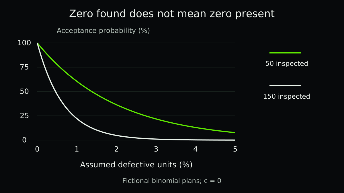
| Assumed defective fraction | n = 50, c = 0 | n = 150, c = 0 |
|---|---|---|
| 0.5% | 77.83% | 47.15% |
| 1% | 60.50% | 22.15% |
| 5% | 7.69% | 0.0456% |
Name both risks rather than choosing a large sample
At a stated good-quality reference, producer’s risk is the probability of rejection. At a stated poor-quality reference, consumer’s risk is the probability of acceptance. The operating-characteristic curve shows acceptance across possible defect fractions. Agree the reference levels and risks before selecting the plan.
For example, at a 1% reference the two plans above reject 39.50% and 77.85% of lots under the model. A stricter rule has an operational cost. AQL is a reference used in a sampling scheme, not permission to ship known bad items or proof of the inspected lot’s quality. Use applicable customer and regulatory requirements; safety-critical decisions need a competent, approved plan.
Use a finite-lot calculation when the approximation matters
Suppose a fictional lot has 100 units, exactly two of them defective, and ten units are sampled randomly without replacement. The probability of finding zero defects is C(98,10) / C(100,10) = 80.91%. The binomial approximation gives 0.98^10 = 81.71%. These are different sampling models.
The exact count of two defectives is assumed to demonstrate the calculation; inspectors normally do not know it. For a specified finite population, use the hypergeometric model when sampling without replacement. Do not turn a convenient percentage-of-lot rule into a sampling plan.
Record the result and decide what happens to the lot
Keep the lot ID, plan revision, random-selection method, inspected unit IDs, actual findings, inspector and disposition. Separate acceptance from release authority: other checks, certificates or holds may still apply. A failed sample should trigger the agreed action, not another sample until one passes.
The downloadable JSON contains the worked probabilities plus a blank decision record. Populate it with your approved plan; do not use the demonstration’s n values as purchasing requirements. Track the cause and cost of rejects separately from first-pass yield.
- Agree the plan
Name the lot, defect definition, risk references, sampling model and authorized disposition.
- Select and inspect
Use the agreed random method, protect traceability and retain the original findings.
- Apply the fixed rule
Record accept, reject or hold without silently changing the rule after seeing results.
- Investigate and review
Follow the response plan and review supplier/process evidence before changing future sampling.
Keep lot acceptance separate from process learning
A lot decision concerns a defined population now. A control chart follows a process over time; process capability compares suitable process data with specifications. Neither substitutes for the other.
The supporting video below introduces control charts, not acceptance-sampling calculations. Use it when deciding how repeated inspection evidence should lead to process investigation. Vrolen is in private pilot; the practical connection is to preserve the decision, its assumptions and what the team learned afterward.
A related example from Abolfazl
Compare a different finite-lot example with acceptance number one.
In English, on founder Abolfazl’s personal blog. This is related reading, not an independent technical source.
Practical checklist
- Define the lot and defect unit.
- Agree n, c and the plan revision before sampling.
- Cover the lot with a defensible random-selection method.
- Check inspection and measurement limitations.
- State the sampling model and risk reference levels.
- Keep actual findings and unit IDs.
- Record the authorized disposition and other holds.
- Follow the rejection response without resampling until a pass.
FAQ
FAQ
Sources and further reading
Authoritative references used to research and verify this guide.