
Little’s Law connects average work in progress, throughput and lead time: WIP = throughput × lead time. For a consistent process boundary, divide average WIP by the average completion rate to estimate average time inside it. Keep units and time bases aligned. A snapshot of today’s queue is not an average. The relationship helps check flow, but it does not prove that removing a particular buffer will preserve output or that an individual order will finish on time.
Calculate lead time with matching units and boundaries.
Replace a queue snapshot with a time-weighted average.
Treat a lower-WIP scenario as a test, not a guaranteed result.
Draw the boundary before using the equation
Work in progress, or WIP, is the material that has entered your chosen process and has not yet left it. For a release-to-final-inspection boundary, include queues, machines, transfers and any rework still inside. Finished goods already outside that boundary do not belong in this WIP count.
Throughput is the completion rate across the same exit. Lead time is the average time a unit spends between that entry and exit, including waiting. MIT’s manufacturing coursework uses Little’s Law to connect these quantities. Mixing whole-factory stock with one machine’s output gives an answer with no clear meaning.
A value stream map helps make the entry, exit and waiting locations explicit.
Use averages measured on one time basis
For long-run stable averages, WIP equals throughput multiplied by lead time. In a finite observation window, arrivals, departures and unfinished work can make a simple estimate misleading. Check whether the window represents normal flow rather than a backlog surge.
Use working hours throughout, or calendar hours throughout. Three working hours is not a promise of delivery three clock hours from now if the line stops overnight. Product units must also match: do not divide kits by individual-part completions.
Units ÷ (units per working hour) = working hours. Use a representative period and the same entry and exit.
Calculate a three-hour flow estimate
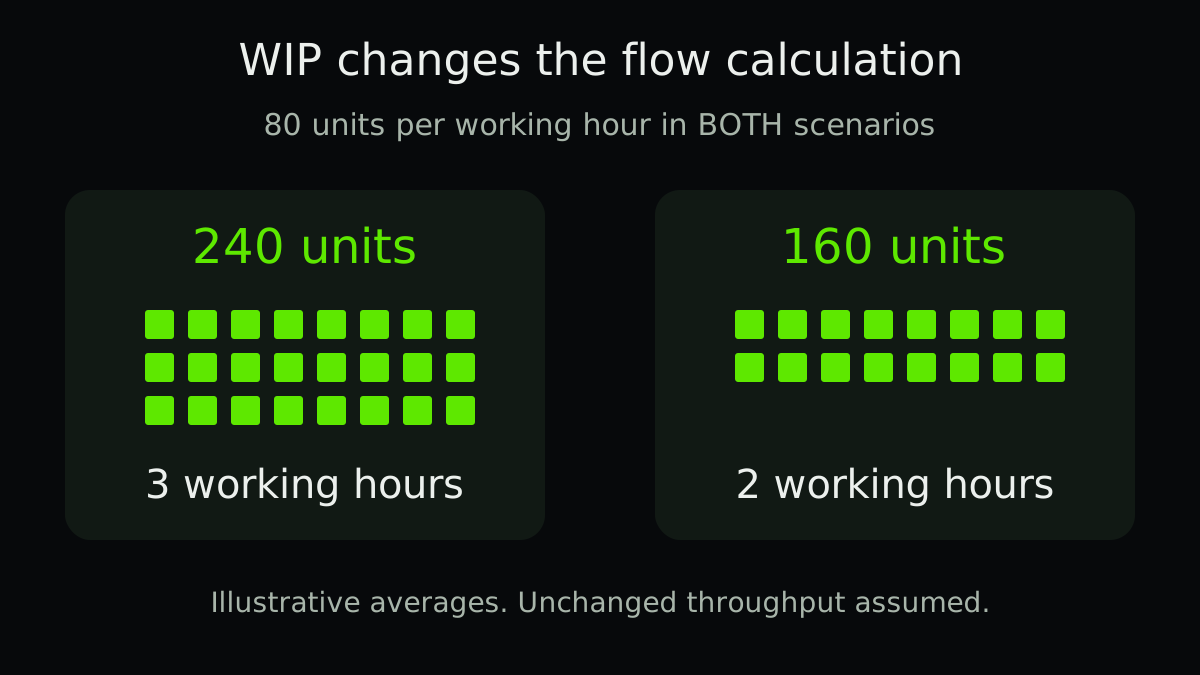
Illustrative stable-flow example: average WIP is 240 units and average throughput is 80 units per working hour. There is no scrap in this example; each unit leaves once as a completed unit. The implied average lead time is 240 ÷ 80 = 3 working hours.
At the same throughput, an average of 160 units would correspond to 2 working hours. That is an arithmetic scenario. It does not tell you whether the actual line can sustain 80 units per hour with less protection against interruptions.
| Illustrative condition | Average WIP | Throughput | Implied mean lead time |
|---|---|---|---|
| Current stable averages | 240 units | 80 units/working h | 3 working h |
| Lower-WIP scenario, same output | 160 units | 80 units/working h | 2 working h |
| Lower WIP, output also drops | 160 units | 60 units/working h | 2.67 working h |
A queue count needs a duration
Suppose WIP stays at 200 units for two hours, then 280 for two hours. The four-hour time-weighted mean is (200 × 2 + 280 × 2) ÷ 4 = 240 units. Using the final count of 280 overstates that period’s mean.
For unequal intervals, weight every count by how long it persisted. A short four-hour average can demonstrate the calculation, but cannot establish long-run stability. Validate the implied lead time with unit entry and exit timestamps over a representative period.
- Specify the unit and boundary
Choose a product family, entry event and completion event. State how scrap and rework exit the system.
- Measure WIP over time
Use event-based duration weighting or regular sampling. Include off-machine queues inside the boundary.
- Calculate completions per hour
Use the same observation window and time basis. Do not count repeated inspections as new units.
- Check the estimate
Compare with actual unit residence times and inspect unfinished orders. Explain any mismatch before changing release rules.
Less inventory can expose a capacity problem
Buffers can keep a constraint supplied during variability upstream. Removing stock indiscriminately may lower output. The Project Production Institute tutorial describes how WIP, variability and throughput interact; its zero-variability reference is not a buffer prescription for a real line.
Start with a bounded release experiment, one product family and an agreed stop condition. Track WIP, good output, starvation, delivery performance and rework together. The production scheduling guide explains why materials and changeovers belong in that test.
Where the estimate needs extra care
A growing backlog means arrivals are outpacing exits. Do not present a short-window WIP ratio as an established long-run lead time. Open orders also matter: averaging only finished fast jobs can make actual residence time look too short.
Scrap is an exit too. If WIP includes units that later scrap, dividing by good-unit output alone mixes populations. Count all relevant exits consistently, or use a separately defined good-unit flow model.
For mixed products, investigate families before pooling averages. Little’s Law can check the consistency of the model; it cannot explain why an individual order waited. Use the lean manufacturing guide to investigate the waiting itself.
Practical checklist
- Name the entry and exit events.
- Use one consistent product or equivalent unit.
- Include all WIP inside the boundary.
- Time-weight queue levels rather than using one snapshot.
- Match the observation period for WIP and throughput.
- Keep working and calendar hours separate.
- Account for scrap, rework and unfinished units.
- Test lower WIP while protecting output and delivery.
FAQ
FAQ
Sources and further reading
Authoritative references used to research and verify this guide.