

Weibull analysis models time to a defined failure using a distribution whose shape can describe different age-related behavior. B10 is the age at which the fitted or assumed model predicts 10% of the population has failed. It is not a guaranteed life or an automatic replacement interval. Include units that have not failed yet as censored observations where appropriate. This assumed-model calculation explains the quantities without claiming to fit a factory’s reliability from a small demonstration.
Separate average life, B10 and conditional age-related failure risk.
Keep still-running units in the reliability record.
Understand the assumptions before selecting a maintenance age.
Define one failure mode and the exposure clock
A time-to-first-failure study needs a clear population, starting point, exposure unit and failure definition. Operating hours, cycles and calendar time answer different questions. Different failure modes or redesigned parts may require separate populations rather than one convenient fitted curve.
NIST distinguishes lifetime models from repairable-system failure-process models. MTBF and MTTR summarize other boundaries; an equipment fleet’s repair events cannot automatically be treated as independent lifetimes of new components.
Read shape and scale without turning them into a story
For a two-parameter Weibull model, reliability is R(t)=exp(−(t/eta)^beta), with t≥0, shape beta>0 and scale eta>0. When beta=1 the hazard is constant; above 1 it increases with age and below 1 it decreases within the model.
Eta is the age at which the model predicts about 63.2% have failed, not the average lifetime. A fitted shape does not prove a physical mechanism. Inspect model fit, population consistency and uncertainty before interpreting it as wear or early-life behavior.
F is cumulative failure probability under the stated lifetime model. Parameters are assumed below, not estimated from the separate sample record.
Calculate B10 for an explicitly assumed model
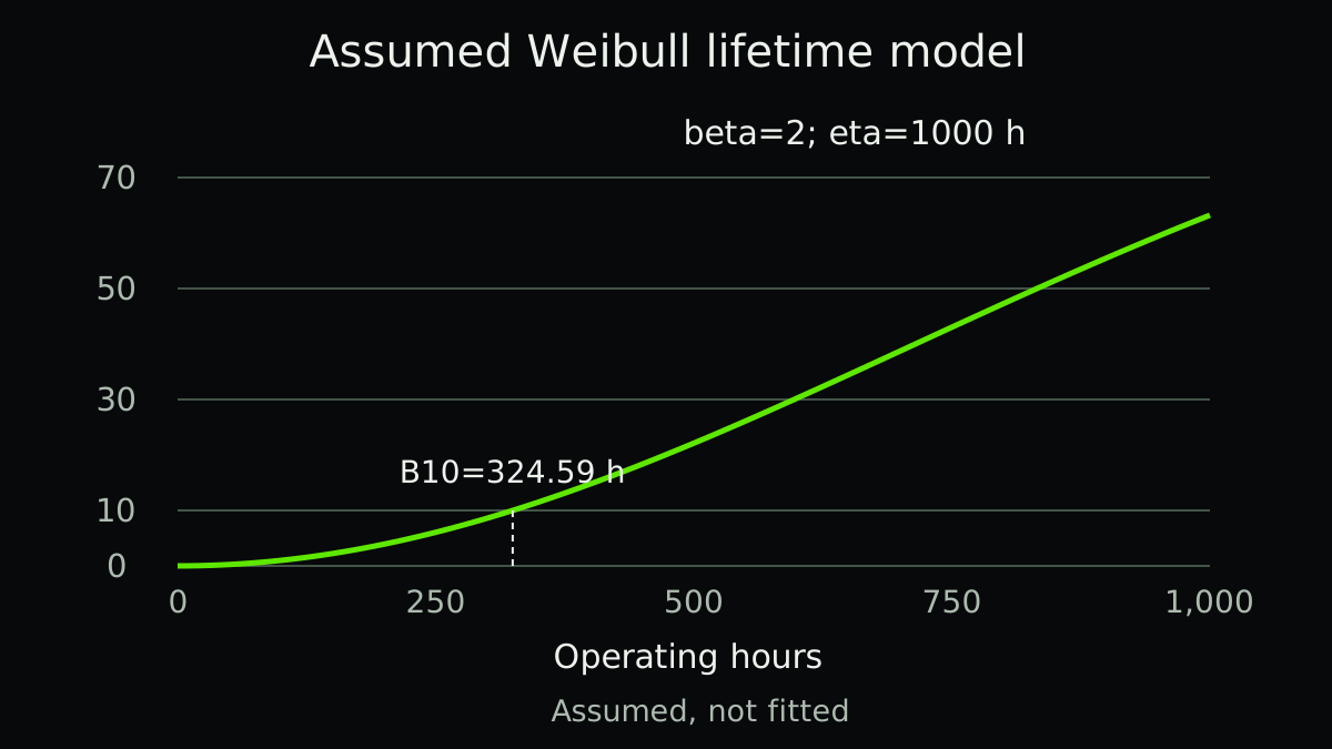
Our illustrative model assumes beta=2 and eta=1000 operating hours. It gives B10=324.59 hours, median life 832.55 hours and mean life 886.23 hours. These are different summaries of the same assumed distribution, not measured plant results.
At 100 hours, the model predicts 0.995% failed; at 1000 hours, 63.212%. The probability of failure during the next 100 hours, conditional on surviving to 900 hours, is 17.304%. Compare that with 0.995% in the first 100 hours. Age matters in this assumed model.
| Quantity | Assumed-model result | Meaning |
|---|---|---|
| B10 | 324.59 h | 10% cumulative failure |
| Median | 832.55 h | 50% cumulative failure |
| Mean | 886.23 h | Expected lifetime, not a guaranteed interval |
| Failure in first 100 h | 0.995% | New unit at time zero |
| Failure from 900 to 1000 h given survival to 900 h | 17.304% | Conditional probability for a surviving unit |
Keep the units that have not failed
In a separate fictional collection record, eight identical new units enter service together. Four fail at 300, 500, 700 and 900 hours; four remain operating when observation stops at 1000 hours. Those four contribute right-censored exposure, not failures at 1000 hours and not missing rows.
NIST provides likelihood methods for censored lifetime data. This article does not fit the assumed beta and eta from that eight-unit record. Excluding surviving units or marking them as failed changes the evidence and can distort the lifetime estimate.
- Define the population and clock
Record component revision, failure mode, start and exposure unit.
- Preserve failures and censored exposure
Store observed age and event status for every included unit.
- Fit and check an appropriate model
Review censoring assumptions, competing modes, fit and interval uncertainty.
- Evaluate the decision separately
Use consequences and task effectiveness rather than treating B10 as a maintenance instruction.
Check censoring and selection assumptions
A unit removed because it already shows deterioration is not equivalent to a randomly still-running observation. Record why observation ended. Truncation, replacements, changed conditions and competing failure modes may require a different analysis.
Avoid estimating a precise replacement policy from a handful of failures. The RCM guide addresses whether an age-based task is applicable, while predictive maintenance asks another question about detectable warning and response.
Publish the model boundary beside the number
A useful reliability record shows the data definition, censoring rules, parameter estimation method, uncertainty and intended decision. Keep a fitted result separate from an assumed scenario. A smooth curve can make weak input evidence look more certain than it is.
The download keeps the assumed-model calculations separate from the eight-unit collection record, to which no model has been fitted. Use the blank fields to record censoring reasons before requesting an analysis. Neither a smooth curve nor this article approves a safety-related replacement age.
A related example from Abolfazl
Compare the same downtime caused by frequent failures or slow recovery.
In English, on founder Abolfazl’s personal blog. This is related reading, not an independent technical source.
Practical checklist
- Define one population and failure mode.
- Choose an exposure clock.
- Record every included unit.
- Distinguish failure from censoring.
- Retain reasons for removal or observation end.
- Separate assumed parameters from fitted estimates.
- Check fit and uncertainty.
- Review consequences before selecting a task or interval.
FAQ
FAQ
Sources and further reading
Authoritative references used to research and verify this guide.