
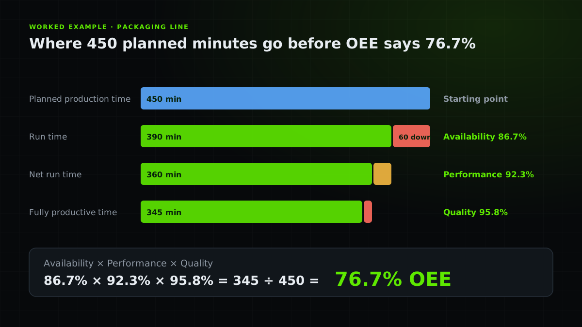
OEE = Availability × Performance × Quality. Availability is run time ÷ planned production time. Performance is (ideal cycle time × total count) ÷ run time. Quality is good count ÷ total count. A line with 450 planned minutes, 390 run minutes, 720 units made and 690 good scores 86.7% × 92.3% × 95.8% = 76.7%. The score shows where time was lost. It does not show whether recovering that time will raise shipments.
A formula you can calculate from four numbers
A worked example with every step shown
A way to map the score to the six big losses
The OEE formula
Overall Equipment Effectiveness compares the time you spent making good product at the ideal rate with the time you planned to produce. It is the product of three factors, and each one answers a different question.
The same score can be written as a single ratio: OEE = (good count × ideal cycle time) ÷ planned production time. The result is identical, but the three-factor version keeps the loss categories apart, and that is what makes OEE useful for improvement.
- Availability: how much of the planned production time did the equipment actually run?
- Performance: while it ran, how close was it to the ideal production rate?
- Quality: how much of the output was good the first time?
Availability = run time ÷ planned production time. Performance = (ideal cycle time × total count) ÷ run time. Quality = good count ÷ total count.
Worked example: a packaging line
A packaging line is planned to produce for 450 minutes. It stops for 60 minutes, so it runs for 390. The ideal cycle time is 0.5 minutes per unit. It makes 720 units, and 690 of them are good the first time.
The rounded factors multiply to 76.6%, but the exact ratio of fully productive time to planned time is 345 ÷ 450 = 76.7%. Carry full precision until the last step, or scores drift by a tenth of a point between spreadsheets.
| Factor | Calculation | Result |
|---|---|---|
| Availability | 390 ÷ 450 | 86.7% |
| Performance | (0.5 × 720) ÷ 390 = 360 ÷ 390 | 92.3% |
| Quality | 690 ÷ 720 | 95.8% |
| OEE | 345 ÷ 450 (fully productive time ÷ planned time) | 76.7% |
Map the score to the six big losses
The three factors tell you which kind of loss dominates. The six big losses split them further, and each one calls for a different response.
A 76.7% OEE produced by long changeovers needs a different response from a 76.7% produced by microstops or reject loss. That is why the number is a starting point for diagnosis, not the diagnosis. Stop-recording rules matter here: short stops below your threshold land in performance, not availability. Read production downtime tracking for how to capture them.
| Factor | Big loss | Typical example |
|---|---|---|
| Availability | 1. Equipment failure | A motor trips and waits for maintenance |
| Availability | 2. Setup and adjustment | Changeover, warm-up and first-piece approval |
| Performance | 3. Small stops | Jams and sensor trips cleared in a minute or two |
| Performance | 4. Reduced speed | Running below the ideal rate to protect quality |
| Quality | 5. Production rejects | Scrap and rework during steady running |
| Quality | 6. Startup rejects | Scrap after a changeover or restart |
Common mistakes when calculating OEE
Most arguments about OEE are arguments about definitions, not arithmetic. These are the mistakes that make two scores incomparable.
- Defining planned production time differently by line or plant, then comparing the scores.
- Taking the ideal cycle time from an old standard or a brochure instead of a defensible best demonstrated rate.
- Mixing planned and unplanned stops, so scheduled breaks show up as availability loss.
- Ignoring stops that fall below the recording threshold, then wondering why performance looks too good.
- Counting reworked units as good, which hides quality loss.
- Averaging OEE across products with different ideal rates instead of calculating per product or weighting by time.
When OEE lies to you: improving the score instead of the system
Suppose the line above is not the constraint. Cutting its changeover by 15 minutes raises OEE, but if a downstream machine limits shipments, the customer receives no extra units. The recovered time becomes idle capacity or inventory.
The same trap appears when teams raise OEE by lengthening batches, loosening the ideal cycle time or recoding stops. Vrolen’s OEE loss analysis guide treats OEE as loss evidence rather than the final target, and why OEE improved but throughput did not covers seven ways the two diverge. Before prioritizing any OEE loss, ask five questions.
- Constraint
Is this resource limiting system output? Start with bottleneck analysis.
- Propagation
Does the loss starve or block another process?
- Output
Would recovering it create sellable output?
- Inventory
Or would it only add stock that waits somewhere else?
- Side effects
What happens to quality and downstream flow?
Practical checklist
- Define planned production time once and apply it to every line.
- Use a defensible ideal cycle time and record where it came from.
- Track planned stops and unplanned stops separately.
- Decide the stop threshold and how short stops are represented.
- Use first-pass good output for quality; never count rework as good.
- Segment by product where ideal rates differ.
- Do not compare plants with different definitions as if the scores were equal.
- Pair OEE with throughput, lead time and demand before deciding what to fix.
FAQ
Questions before you join
Sources and further reading
Authoritative references used to research and verify this guide.