

Validate a manufacturing simulation against operating evidence relevant to the decision it will support. First verify that the implementation follows the intended rules, then compare outputs with independent periods under matched conditions. Check throughput, queues, lead time and resource behaviour, not just one average. Define acceptance criteria before tuning, quantify important uncertainty and document where the model does not apply. A model that fits one historical period is not automatically credible for a changed line.
Separate implementation verification from real-world validation.
Detect a misleading aggregate match in a worked example.
Define the conditions under which a scenario deserves trust.
Start with the decision and its consequence
A model used to compare buffer sizes needs different evidence from one used to commit a delivery date. Name the proposed decision, feasible alternatives and the cost of choosing incorrectly.
NIST’s manufacturing digital-twin credibility work treats verification, validation and uncertainty as ongoing activities. The principle applies to a discrete-event production simulation even if it is not connected to live equipment.
The digital twin, simulation and process-mining comparison helps choose the approach. This companion checks whether a chosen model supports a particular decision.
Verify the implementation before comparing averages
Trace a single unit through a simple run. Check routing, resource seizure and release, setup logic, calendars and failure recovery. Units should not disappear, multiply or occupy the same exclusive resource simultaneously.
For a simple system boundary, starting WIP plus entrants should equal departures plus ending WIP, with scrap and other exits accounted for. Test closed periods, zero demand, a blocked downstream process and a stopped constraint.
An animation can look convincing while using the wrong calendar or allowing an impossible resource overlap. Retain event traces and explicit test cases, not just screenshots.
An aggregate match can hide the wrong days
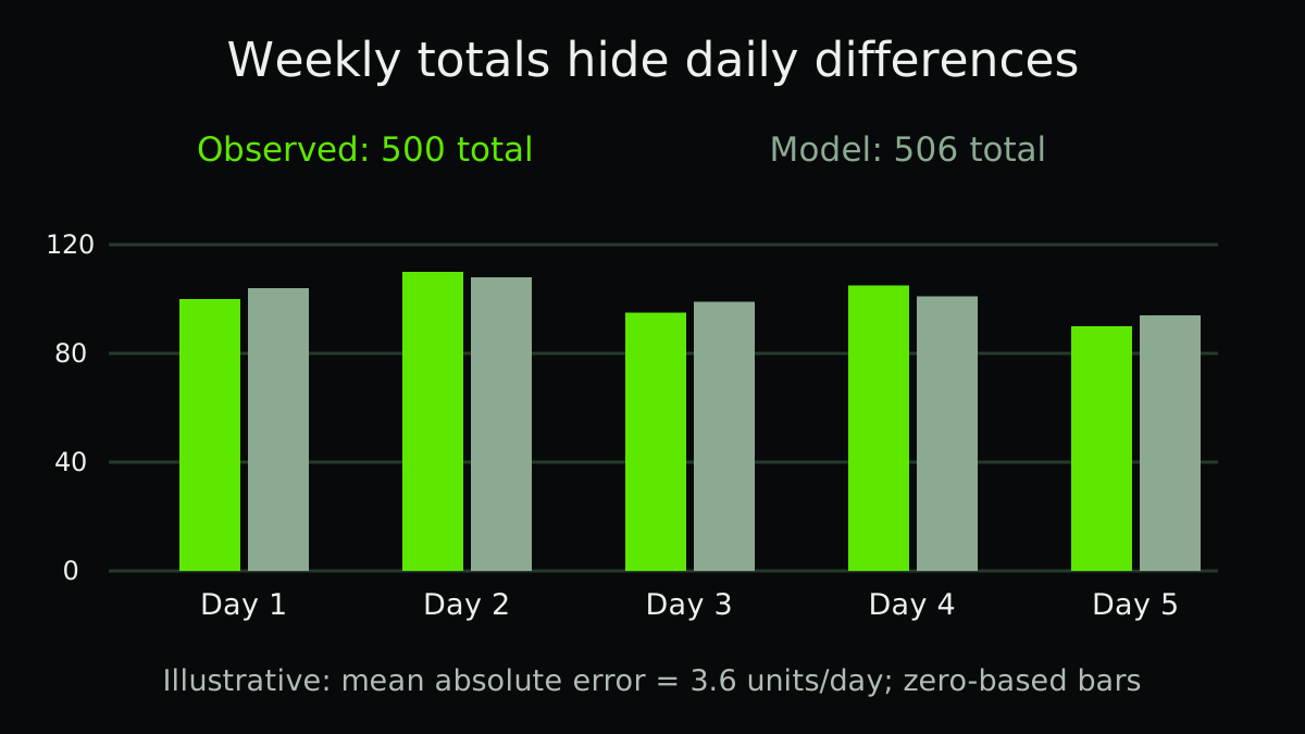
Illustrative matched five-day period: observed good output is 100, 110, 95, 105 and 90 units. A model gives 104, 108, 99, 101 and 94. Observed total is 500; model total is 506, only 1.2% higher.
Daily absolute errors are 4, 2, 4, 4 and 4 units. Mean absolute error is 18 / 5 = 3.6 units per day. A close weekly total does not establish that the model describes the day-level operating pattern, queue or delivery risk.
These five results demonstrate calculation, not enough stochastic replications or validation coverage. A real assessment needs repeated runs where random inputs matter and independent operating conditions.
| Day | Observed units | Model units | Absolute error |
|---|---|---|---|
| 1 | 100 | 104 | 4 |
| 2 | 110 | 108 | 2 |
| 3 | 95 | 99 | 4 |
| 4 | 105 | 101 | 4 |
| 5 | 90 | 94 | 4 |
| Total | 500 | 506 | 18 summed absolute errors |
Keep fitting data separate from validation data
Use one period to estimate inputs and tune the model, then hold out other periods for comparison. Match product mix, staffing, planned time, starting WIP and material availability. A model of one shift is not fairly judged against another shift’s workload.
Record warm-up treatment and starting state. An empty simulated line can behave differently from a plant that begins with full buffers. For stochastic simulations, retain seeds, replications and interval estimates.
NIST’s SimPROCESD work provides an open discrete-event manufacturing example with explicit production-system features. Software availability is not evidence that your particular model has been validated.
- Agree acceptance before tuning
Choose decision-relevant outputs, error measures, intervals and operating conditions with the decision owner.
- Verify rules with small tests
Check resource conflicts, conservation, calendars, disruptions and route logic using inspectable event traces.
- Compare held-out operation
Run matched conditions and compare output, queue distributions, lead time and resource behaviour.
- Test uncertainty and limits
Vary important uncertain inputs, repeat stochastic runs and document where the recommendation changes.
Validate the mechanism that drives the recommendation
If the model recommends another machine, inspect the predicted constraint, starvation and blocking against observed evidence. Matching total output with unrealistic queue behaviour can support the wrong investment.
Use bottleneck analysis to identify the physical evidence. Seek operator and planner review of the rules, especially interruptions and informal workarounds absent from system logs.
A scenario introduces conditions not directly observed. Validate relevant components and use sensitivity analysis; do not call the new scenario proven simply because the baseline fitted.
Treat credibility as versioned evidence
Store input datasets, assumptions, model revision, run settings, tests, limitations and acceptance decisions together. When routing, setup or staffing changes, revisit the evidence affected.
Report a recommendation as conditional on the validated boundary and uncertainty. A digital twin that refreshes data continuously still needs review when the process or model changes.
Practical checklist
- Name the decision and consequence of error.
- Agree acceptance criteria before tuning.
- Verify routing, resources and conservation.
- Match calendars, mix and starting state.
- Keep independent held-out periods.
- Compare queues and lead time as well as throughput.
- Record stochastic replications and input uncertainty.
- Version evidence and state where the model does not apply.
FAQ
FAQ
Sources and further reading
Authoritative references used to research and verify this guide.